Posts
Tables are also a part of data visualization. Elegant tables may make your article better for the editors/reviewers.
Selected article:
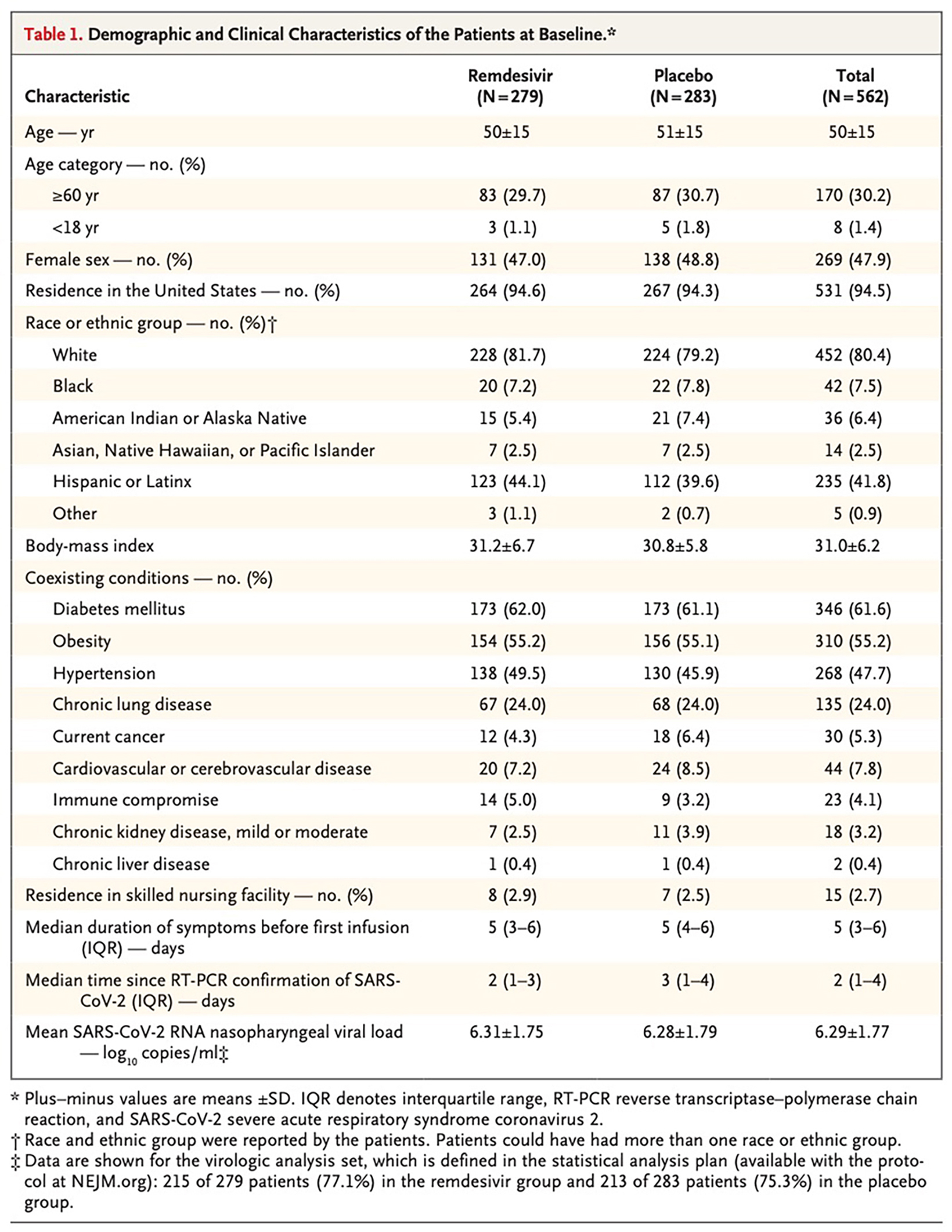
Title: Early Remdesivir to Prevent Progression to Severe Covid-19 in Outpatients
Journal: The New England Journal of Medicine
Authors: Gottlieb RL, Vaca CE, Paredes R, et al.
Year: 2022
PMID: 34937145
DOI: 10.1056/NEJMoa2116846
The original figure
Import libraries
library(tidyverse)
library(fabricatr)      # to fabricate fake data

library(finalfit)       # to create final output tables
library(flextable)      # to create/modify/format tables for reporting and publications
library(ftExtra)        # extensions for flextable package
library(officer)        # to manipulate Word document
Prepare fabricated data
set.seed(2022)
group_remdecivir <- fabricate(
  N = 279,
  age = round(rnorm(N, mean = 50, sd = 15)),
  bmi = round(rnorm(N, mean = 31.2, sd = 6.7), 1),
  dur_symptoms = round(runif(N, min = 1.5, max = 8)),
  dur_since_sirs = round(runif(N, min = 0, max = 4)),
  viral_load = round(rnorm(N, mean = 6.31, sd = 1.75), 3),
  sex = draw_binary(N = N, prob = 0.53),
  residence_usa = draw_binary(N = N, prob = .946),
  white = draw_binary(N = N, prob = 0.817),
  black = draw_binary(N = N, prob = 0.072),
  american_indian_native = draw_binary(N = N, prob = 0.054),
  asian_native = draw_binary(N = N, prob = 0.025),
  hispanic = draw_binary(N = N, prob = 0.441),
  other = draw_binary(N = N, prob = 0.011),
  diabetes = draw_binary(N = N, prob = .62),
  obesity = draw_binary(N = N, prob = .552),
  ht = draw_binary(N = N, prob = .495),
  lung = draw_binary(N = N, prob = .24),
  cancer = draw_binary(N = N, prob = .043),
  cardiac = draw_binary(N = N, prob = .072),
  immune = draw_binary(N = N, prob = .05),
  kidney = draw_binary(N = N, prob = .025),
  liver = draw_binary(N = N, prob = .004),
  residence_nursing = draw_binary(N = N, prob = 0.029),
  group = "Remdesivir") %>%
  as_tibble()


set.seed(2022)
group_placebo <- fabricate(
  N = 283,
  age = round(rnorm(N, mean = 51, sd = 15)),
  bmi = round(rnorm(N, mean = 30.8, sd = 5.8), 1),
  dur_symptoms = round(runif(N, min = 2, max = 8)),
  dur_since_sirs = round(runif(N, min = 0, max = 5)),
  viral_load = round(rnorm(N, mean = 6.28, sd = 1.79), 3),
  sex = draw_binary(N = N, prob = 0.512),
  residence_usa = draw_binary(N = N, prob = .943),
  white = draw_binary(N = N, prob = 0.792),
  black = draw_binary(N = N, prob = 0.078),
  american_indian_native = draw_binary(N = N, prob = 0.074),
  asian_native = draw_binary(N = N, prob = 0.025),
  hispanic = draw_binary(N = N, prob = 0.396),
  other = draw_binary(N = N, prob = 0.007),
  diabetes = draw_binary(N = N, prob = .611),
  obesity = draw_binary(N = N, prob = .551),
  ht = draw_binary(N = N, prob = .459),
  lung = draw_binary(N = N, prob = .24),
  cancer = draw_binary(N = N, prob = .064),
  cardiac = draw_binary(N = N, prob = .085),
  immune = draw_binary(N = N, prob = .032),
  kidney = draw_binary(N = N, prob = .039),
  liver = draw_binary(N = N, prob = .004),
  residence_nursing = draw_binary(N = N, prob = 0.025),
  group = "Placebo"
  ) %>%
  as_tibble()


combined_dataset <- bind_rows(group_remdecivir, group_placebo)  %>%
  mutate (patient_id = paste0("P_", row_number())) %>%
  select(patient_id, group, everything(), -ID) %>%
  mutate(group = fct_relevel(group, "Remdesivir", "Placebo"),
         age_category_over60 = factor(if_else(age >= 60, "yes", "no")),
         age_category_under18 = factor(if_else(age < 18, "yes", "no"))) %>%
  mutate_if(is.integer, as.factor) %>%
  mutate(sex = fct_recode(sex, "female" = "0", "male" = "1")) %>%
  mutate(across((residence_usa:residence_nursing), ~ fct_recode(., "no" = "0", "yes" = "1"))) %>%
  add_column(age_category = "yes",      # I added three columns. This is my trick to add empty rows into the table. We can merge them in flextable step.
             race_ethnic = "yes",
             comorbidities = "yes")
Possible strategy: Tables are good to present the exact data. but not that good as an informative figure, however, they are needed to present scientific data. I always use {finalfit} package to prepare my tables. It is life-saver and saved my hours-days in my projects. Not only table-1, also great for logistic regression, Cox regression, multilevel/multivariable analysis.
After I realized that finalfit object is a data.frame, I added all tidyverse tricks to improve my tables with R codes. Because Microsoft Word file is used to submit our papers, I added {flextable}, {officer}, {ftExtra} packages into my workflow. Although there are other tools to present tables in R, {flextable} seems the best for a word output.
R codes for the table
explanatory <-  combined_dataset %>%
  select(age, age_category, age_category_over60, age_category_under18, sex, residence_usa, race_ethnic, white:other, bmi,comorbidities, diabetes:residence_nursing, dur_symptoms:viral_load) %>%
  names()

dependent <- "group"

finalfit_table <- combined_dataset %>%
  mutate(across(c(age_category_over60, age_category_under18, residence_usa:residence_nursing), ~fct_relevel(., "yes", "no"))) %>%       # This is my trick to remove "no" rows in the flextable step.
  summary_factorlist(dependent = dependent,
                     explanatory = explanatory,
                     p = FALSE,
                     cont_nonpara = c(26, 27),
                     total_col = TRUE,
                     add_col_totals = TRUE,
                     include_col_totals_percent = FALSE,
                     col_totals_prefix = "N=")
output of finalfit package
finalfit_table %>%
        knitr::kable() %>% kableExtra::kable_styling()
| label | levels | Remdesivir | Placebo | Total |
|---|---|---|---|---|
| Total N | N=279 | N=283 | N=562 | |
| age | Mean (SD) | 49.7 (15.0) | 50.6 (15.0) | 50.2 (15.0) |
| age_category | yes | 279 (100.0) | 283 (100.0) | 562 (100.0) |
| age_category_over60 | yes | 78 (28.0) | 80 (28.3) | 158 (28.1) |
| no | 201 (72.0) | 203 (71.7) | 404 (71.9) | |
| age_category_under18 | yes | 2 (0.7) | 1 (0.4) | 3 (0.5) |
| no | 277 (99.3) | 282 (99.6) | 559 (99.5) | |
| sex | female | 128 (45.9) | 143 (50.5) | 271 (48.2) |
| male | 151 (54.1) | 140 (49.5) | 291 (51.8) | |
| residence_usa | yes | 263 (94.3) | 267 (94.3) | 530 (94.3) |
| no | 16 (5.7) | 16 (5.7) | 32 (5.7) | |
| race_ethnic | yes | 279 (100.0) | 283 (100.0) | 562 (100.0) |
| white | yes | 216 (77.4) | 218 (77.0) | 434 (77.2) |
| no | 63 (22.6) | 65 (23.0) | 128 (22.8) | |
| black | yes | 21 (7.5) | 26 (9.2) | 47 (8.4) |
| no | 258 (92.5) | 257 (90.8) | 515 (91.6) | |
| american_indian_native | yes | 19 (6.8) | 19 (6.7) | 38 (6.8) |
| no | 260 (93.2) | 264 (93.3) | 524 (93.2) | |
| asian_native | yes | 7 (2.5) | 5 (1.8) | 12 (2.1) |
| no | 272 (97.5) | 278 (98.2) | 550 (97.9) | |
| hispanic | yes | 117 (41.9) | 110 (38.9) | 227 (40.4) |
| no | 162 (58.1) | 173 (61.1) | 335 (59.6) | |
| other | yes | 5 (1.8) | 1 (0.4) | 6 (1.1) |
| no | 274 (98.2) | 282 (99.6) | 556 (98.9) | |
| bmi | Mean (SD) | 31.0 (6.8) | 30.6 (5.9) | 30.8 (6.4) |
| comorbidities | yes | 279 (100.0) | 283 (100.0) | 562 (100.0) |
| diabetes | yes | 171 (61.3) | 173 (61.1) | 344 (61.2) |
| no | 108 (38.7) | 110 (38.9) | 218 (38.8) | |
| obesity | yes | 144 (51.6) | 143 (50.5) | 287 (51.1) |
| no | 135 (48.4) | 140 (49.5) | 275 (48.9) | |
| ht | yes | 133 (47.7) | 112 (39.6) | 245 (43.6) |
| no | 146 (52.3) | 171 (60.4) | 317 (56.4) | |
| lung | yes | 62 (22.2) | 61 (21.6) | 123 (21.9) |
| no | 217 (77.8) | 222 (78.4) | 439 (78.1) | |
| cancer | yes | 9 (3.2) | 13 (4.6) | 22 (3.9) |
| no | 270 (96.8) | 270 (95.4) | 540 (96.1) | |
| cardiac | yes | 13 (4.7) | 25 (8.8) | 38 (6.8) |
| no | 266 (95.3) | 258 (91.2) | 524 (93.2) | |
| immune | yes | 14 (5.0) | 9 (3.2) | 23 (4.1) |
| no | 265 (95.0) | 274 (96.8) | 539 (95.9) | |
| kidney | yes | 7 (2.5) | 10 (3.5) | 17 (3.0) |
| no | 272 (97.5) | 273 (96.5) | 545 (97.0) | |
| liver | yes | 2 (0.7) | 2 (0.7) | 4 (0.7) |
| no | 277 (99.3) | 281 (99.3) | 558 (99.3) | |
| residence_nursing | yes | 8 (2.9) | 8 (2.8) | 16 (2.8) |
| no | 271 (97.1) | 275 (97.2) | 546 (97.2) | |
| dur_symptoms | Median (IQR) | 5.0 (3.0 to 6.0) | 5.0 (4.0 to 6.0) | 5.0 (3.0 to 6.0) |
| dur_since_sirs | Median (IQR) | 2.0 (1.0 to 3.0) | 3.0 (1.0 to 4.0) | 2.0 (1.0 to 3.0) |
| viral_load | Mean (SD) | 6.4 (1.9) | 6.4 (1.9) | 6.4 (1.9) |
modifying finalfit output using tidyverse approach
modified_finalfit_table <- finalfit_table %>%
  dplyr::mutate(across((Remdesivir:Total), ~ if_else(label == "Total N", paste0("(", . , ")"), .))) %>%
  dplyr::mutate(across((Remdesivir:Total), ~ if_else(label %in% c("age", "bmi", "viral_load"), str_replace_all(., " \\(", "±"), . ))) %>%
  dplyr::mutate(across((Remdesivir:Total), ~ if_else(label %in% c("age", "bmi", "viral_load"), str_replace_all(., "\\)", ""), . ))) %>%
  filter(levels != "no") %>%
  filter(levels != "male") %>%
  mutate(levels = if_else(levels %in% c("Median (IQR)", "Mean (SD)"), " ", levels),
         across(Remdesivir:Total, ~str_replace_all(., " to ", "-")), # , "Total" were removed.
         across(Remdesivir:Total, ~str_replace_all(., "\\.0", "")), # , "Total" were removed.
         levels = str_remove_all(levels, "yes"),
         label = fct_recode(label,
                             "Characteristic" = "Total N",
                             "Age—yr" = "age",
                             "≥60 yr" = "age_category_over60",
                             "<18 yr" = "age_category_under18",
                             "Female sex — no. (%)" = "sex",
                             "Residence in the United States — no. (%)" = "residence_usa",
                             "White" = "white",
                             "Black" = "black",
                             "American Indian or Alaska Native" = "american_indian_native",
                             "Asian, Native Hawaiian, or Pacific Islander" = "asian_native",
                             "Hispanic or Latinx" = "hispanic",
                             "Other" = "other",
                             "Body-mass index" = "bmi",
                             "Diabetes mellitus" = "diabetes",
                             "Obesity" = "obesity",
                             "Hypertension" = "ht",
                             "Chronic lung disease" = "lung",
                             "Current cancer" = "cancer",
                             "Cardiovascular or cerebrovascular disease" = "cardiac",
                             "Immune compromise" = "immune",
                             "Chronic kidney disease, mild or moderate" = "kidney",
                             "Chronic liver disease" = "liver",
                             "Residence in skilled nursing facility — no. (%)" = "residence_nursing",
                             "Median duration of symptoms before first infusion (IQR) — days" = "dur_symptoms",
                             "Median time since RT-PCR confirmation of SARS-CoV-2 (IQR) — days" = "dur_since_sirs",
                             "Mean SARS-CoV-2 RNA nasopharyngeal viral load — log~10~ copies/ml" = "viral_load")) %>%
  select(-levels)

modified_finalfit_table %>%
        knitr::kable() %>% kableExtra::kable_styling()
| label | Remdesivir | Placebo | Total |
|---|---|---|---|
| Characteristic | (N=279) | (N=283) | (N=562) |
| Age—yr | 49.7±15 | 50.6±15 | 50.2±15 |
| age_category | 279 (100) | 283 (100) | 562 (100) |
| ≥60 yr | 78 (28) | 80 (28.3) | 158 (28.1) |
| <18 yr | 2 (0.7) | 1 (0.4) | 3 (0.5) |
| Female sex — no. (%) | 128 (45.9) | 143 (50.5) | 271 (48.2) |
| Residence in the United States — no. (%) | 263 (94.3) | 267 (94.3) | 530 (94.3) |
| race_ethnic | 279 (100) | 283 (100) | 562 (100) |
| White | 216 (77.4) | 218 (77) | 434 (77.2) |
| Black | 21 (7.5) | 26 (9.2) | 47 (8.4) |
| American Indian or Alaska Native | 19 (6.8) | 19 (6.7) | 38 (6.8) |
| Asian, Native Hawaiian, or Pacific Islander | 7 (2.5) | 5 (1.8) | 12 (2.1) |
| Hispanic or Latinx | 117 (41.9) | 110 (38.9) | 227 (40.4) |
| Other | 5 (1.8) | 1 (0.4) | 6 (1.1) |
| Body-mass index | 31±6.8 | 30.6±5.9 | 30.8±6.4 |
| comorbidities | 279 (100) | 283 (100) | 562 (100) |
| Diabetes mellitus | 171 (61.3) | 173 (61.1) | 344 (61.2) |
| Obesity | 144 (51.6) | 143 (50.5) | 287 (51.1) |
| Hypertension | 133 (47.7) | 112 (39.6) | 245 (43.6) |
| Chronic lung disease | 62 (22.2) | 61 (21.6) | 123 (21.9) |
| Current cancer | 9 (3.2) | 13 (4.6) | 22 (3.9) |
| Cardiovascular or cerebrovascular disease | 13 (4.7) | 25 (8.8) | 38 (6.8) |
| Immune compromise | 14 (5) | 9 (3.2) | 23 (4.1) |
| Chronic kidney disease, mild or moderate | 7 (2.5) | 10 (3.5) | 17 (3) |
| Chronic liver disease | 2 (0.7) | 2 (0.7) | 4 (0.7) |
| Residence in skilled nursing facility — no. (%) | 8 (2.9) | 8 (2.8) | 16 (2.8) |
| Median duration of symptoms before first infusion (IQR) — days | 5 (3-6) | 5 (4-6) | 5 (3-6) |
| Median time since RT-PCR confirmation of SARS-CoV-2 (IQR) — days | 2 (1-3) | 3 (1-4) | 2 (1-3) |
| Mean SARS-CoV-2 RNA nasopharyngeal viral load — log~10~ copies/ml | 6.4±1.9 | 6.4±1.9 | 6.4±1.9 |
final touch with flextable
set_flextable_defaults(
        font.family = "Open Sans",
        font.size = 10,
        padding.bottom = 3,
        padding.top = 3,
        padding.left = 3,
        padding.right = 3)

table_1 <- modified_finalfit_table %>%
  flextable() %>%
  add_header_lines("[Table 1.]{color=#BD272E} Demographic and Clinical Characteristics of the Patients at Baseline.") %>%
  align(part = "all", align = "center", j=2:ncol(modified_finalfit_table)) %>%
  border_remove(.) %>%
  hline(part="header", i = 1) %>%
  hline_bottom(part="body", border = fp_border(color="black")) %>%
  hline_top(part="header", border = fp_border(color="black")) %>%
  vline_left(border = fp_border(color="black")) %>%
  vline_right(border = fp_border(color="black")) %>%
  bold(part="header", i = 1:2) %>%
  bold(part="body", i = 1) %>%
  padding( part = "body", j = 1, i = c(4,5,9:14,17:25), padding.left = 30) %>%
  bg(bg = "#FFF8E7", part = "body", i=seq(2,nrow(modified_finalfit_table), 2)) %>%
  bg(bg = "#F5EFE7", part = "header", i=1) %>%
  colformat_md(j = 1,  part = "body") %>%
  colformat_md(j = 1, part = "header") %>%
  set_header_labels(i = 1, "label"=" ") %>%
  compose(i = 3, j=1:ncol(modified_finalfit_table),  value = as_paragraph("Age category — no. (%)"), part = "body") %>%
  merge_h (i = 3) %>%
  compose(i = 8, j=1:ncol(modified_finalfit_table),  value = as_paragraph("Race or ethnic group — no. (%)"), part = "body") %>%
  merge_h (i = 8) %>%
  compose(i = 16, j=1:ncol(modified_finalfit_table),  value = as_paragraph("Coexisting conditions — no. (%)"), part = "body") %>%
  merge_h (i = 16) %>%
  footnote(part = "header", i = 1, value = as_paragraph("Plus–minus values are means ±SD. IQR denotes interquartile range, RT-PCR reverse transcriptase–polymerase chain reaction, and SARS-CoV-2 severe acute respiratory syndrome coronavirus 2."), ref_symbols = "\U2606") %>%
  footnote(part = "body", i = 7, j = 1, value = as_paragraph("Race and ethnic group were reported by the patients. Patients could have had more than one race or ethnic group."), ref_symbols = "\U2020") %>%
  footnote(part = "body", i = 29, j = 1, value = as_paragraph("Data are shown for the virologic analysis set, which is defined in the statistical analysis plan (available with the protocol at NEJM.org): 215 of 279 patients (77.1%) in the remdesivir group and 213 of 283 patients (75.3%) in the placebo group."), ref_symbols = "\U2021") %>%
  hline_bottom(part="footer", border = fp_border(color="black")) %>%
  width(j = 1, 8.6, "cm") %>%
  width(j = 2:4, 3.6, "cm") %>%
  fix_border_issues()

# table_1
save flextable object as a word file (portrait or landscape)
sect_properties_portrait <- prop_section(
  page_size = page_size(orient = "portrait",
    width = 11.7, height = 8.3),
  type = "nextPage",
  page_margins = page_mar()
)

save_as_docx(table_1,
             path = here::here("content", "blog", "2022-02-07-week-4",paste0("table_1", ".docx")),
              pr_section = sect_properties_portrait)
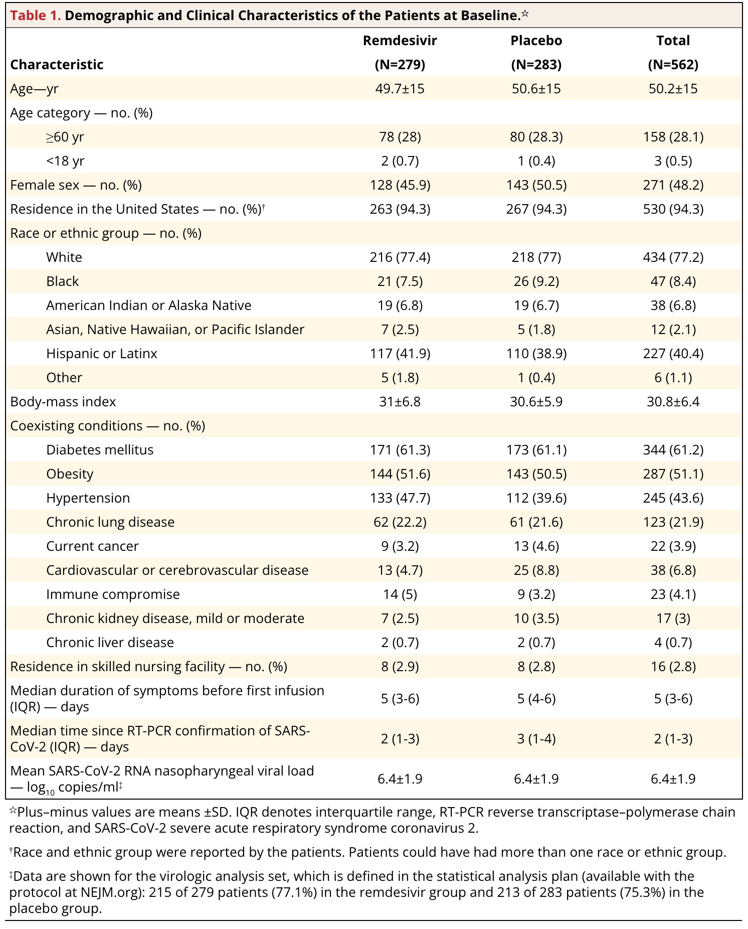
Final replica
Some personal comments:
- finalfit output is good enough. However, because we prefer .docx output for the submission process, It may be a good idea to modify it with code. It gives you reproducibility. flextable and ftExtra is great complements to finalfit output.
- If a word file has more than two pages, It gives repeated header to each pages in word file. No solution via R, however, can be changed in word’s table properties-> Row-> Uncheck “Repeat as header at the top of each page”.
Citation
Ali Guner (Feb 7, 2022) Week-4. Retrieved from https://datavizmed.com/blog/2022-02-07-week-4/
@misc{ 2022-week-4,
author = { Ali Guner },
title = { Week-4 },
url = { https://datavizmed.com/blog/2022-02-07-week-4/ },
year = { 2022 }
updated = { Feb 7, 2022 }
}