Posts
Another table with the power of finalfit and flextable packages.
This time it includes uni- and multi-variable “REGRESSION” analysis.
It is all automated.
Selected article:
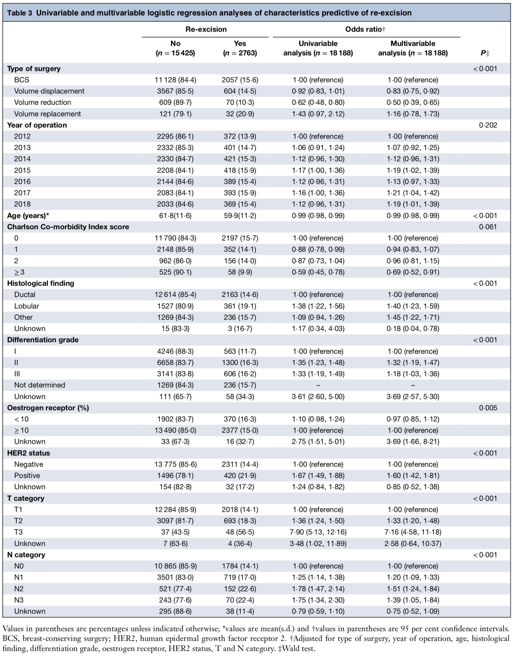
Title: Rates of re-excision and conversion to mastectomy after breast-conserving surgery with or without oncoplastic surgery: a nationwide population-based study
Journal: British Journal of Surgery
Authors: Heeg E, Jensen MB, Hölmich LR, et al.
Year: 2020
PMID: 32761931
DOI: 10.1002/bjs.11838
The original table
Import libraries
library(tidyverse)
library(scales)
library(fabricatr)

library(finalfit)
library(flextable)
library(officer)
Prepare fabricated data
set.seed(2022)
group_no_reexcision <- fabricate(
  N = 15425,
  group = "no reexcision",
  type_of_surgery = c(rep("BCS", 11128), rep("Volume displacement", 3567), rep("Volume reduction", 609), rep("Volume replacement", 121)),
  year = c(rep("2012", 2295), rep("2013", 2332), rep("2014", 2330), rep("2015", 2208), rep("2016", 2144), rep("2017", 2083), rep("2018", 2033)),
  age = round(rnorm(N, mean = 61.8, sd = 11.6), 2),
  charlson = c(rep("0", 11790), rep("1", 2148), rep("2", 962), rep("≥3", 525)),
  histology = c(rep("Ductal", 12614), rep("Lobuler", 1527), rep("Other", 1269), rep("Unknown", 15)),
  diff = c(rep("I", 4246), rep("II", 6658), rep("III", 3141), rep("Not determined", 1269), rep("Unknown", 111)),
  oestrogen = c(rep("<10", 1902), rep("≥10", 13490), rep("Unknown", 33)),
  her2 = c(rep("Negative", 13775), rep("Positive", 1496), rep("Unknown", 154)),
  t_stage = c(rep("T1", 12284), rep("T2", 3097), rep("T3", 37), rep("Unknown", 7)),
  n_stage = c(rep("N0", 10865), rep("N1", 3501), rep("N2", 521), rep("N3", 243), rep("Unknown", 295)))  %>%
  as_tibble() %>%
  mutate(across(type_of_surgery:n_stage, sample)) # This is to shuffle the dataset without changing proportions

set.seed(2022)
group_reexcision <- fabricate(
  N = 2763,
  group = "reexcision",
  type_of_surgery = c(rep("BCS", 2057), rep("Volume displacement", 604), rep("Volume reduction", 70), rep("Volume replacement", 32)),
  year = c(rep("2012", 372), rep("2013", 401), rep("2014", 421), rep("2015", 418), rep("2016", 389), rep("2017", 393), rep("2018", 369)),
  age = round(rnorm(N, mean = 59.9, sd = 11.2), 2),
  charlson = c(rep("0", 2197), rep("1", 352), rep("2", 156), rep("≥3", 58)),
  histology = c(rep("Ductal", 2163), rep("Lobuler", 361), rep("Other", 236), rep("Unknown", 3)),
  diff = c(rep("I", 563), rep("II", 1300), rep("III", 606), rep("Not determined", 236), rep("Unknown", 58)),
  oestrogen = c(rep("<10", 370), rep("≥10", 2377), rep("Unknown", 16)),
  her2 = c(rep("Negative", 2311), rep("Positive", 420), rep("Unknown", 32)),
  t_stage = c(rep("T1", 2018), rep("T2", 693), rep("T3", 48), rep("Unknown", 4)),
  n_stage = c(rep("N0", 1784), rep("N1", 719), rep("N2", 152), rep("N3", 70), rep("Unknown", 38)))  %>%
  as_tibble() %>%
  mutate(across(type_of_surgery:n_stage, sample)) # This is to shuffle the dataset without changing proportions


set.seed(2022)
combined_dataset <-  bind_rows(group_no_reexcision, group_reexcision)  %>%
  as_tibble() %>%
  mutate (patient_id = paste0("P_", row_number())) %>%
  select(patient_id, group, everything(), -ID) %>%
  mutate_if(is_character, factor) %>%
  mutate(patient_id = as.character(patient_id),
         group = fct_relevel(group, "no reexcision", "reexcision"),
         type_of_surgery = fct_relevel(type_of_surgery, "BCS", "Volume displacement", "Volume reduction", "Volume replacement"),
         charlson = fct_relevel(charlson, "0", "1", "2", "≥3"))
A part of fake dataset
## # A tibble: 10 × 12
## patie…¹ group type_…² year age charl…³ histo…⁴ diff oestr…⁵ her2 t_stage
## <chr> <fct> <fct> <fct> <dbl> <fct> <fct> <fct> <fct> <fct> <fct>
## 1 P_9651 no r… BCS 2012 55.4 2 Ductal II ≥10 Posi… T1
## 2 P_7886 no r… BCS 2016 49.0 0 Ductal Not … ≥10 Nega… T1
## 3 P_2871 no r… BCS 2015 43.3 1 Ductal I ≥10 Nega… T1
## 4 P_12107 no r… BCS 2014 44.6 0 Lobuler II ≥10 Nega… T1
## 5 P_8900 no r… Volume… 2015 57.5 0 Ductal II ≥10 Nega… T2
## 6 P_4870 no r… Volume… 2012 55.7 0 Ductal III ≥10 Nega… T1
## 7 P_2751 no r… BCS 2016 51.8 0 Ductal II <10 Nega… T1
## 8 P_16860 reex… BCS 2014 73.8 0 Ductal III ≥10 Nega… T1
## 9 P_123 no r… BCS 2017 71.2 0 Ductal II ≥10 Nega… T1
## 10 P_10473 no r… Volume… 2017 61.3 0 Ductal I ≥10 Nega… T1
## # … with 1 more variable: n_stage <fct>, and abbreviated variable names
## # ¹patient_id, ²type_of_surgery, ³charlson, ⁴histology, ⁵oestrogen
Possible strategy:
I ll use similar approach as was done in Week 4.
The major problem in the table is adding wald test results.
I ll do this with the tidyverse approach as well as the finalfit package.
regTermTest from {survey} can also be used for Wald test.
R codes for the table (the power of finalfit package)
explanatory <-  combined_dataset %>%
  select(type_of_surgery,  year , age, charlson, histology, diff, oestrogen, her2, t_stage, n_stage) %>%
  names()

dependent <- "group"

finalfit_table <- combined_dataset %>%
  finalfit(dependent = dependent,
           explanatory = explanatory,
           add_dependent_label = FALSE,
           column = FALSE)

# finalfit_table


### Wald test results is not included in formal analysis. Because they are in the table, we should calculate them in another analysis (surely with finalfit package)
wald_table <- combined_dataset %>%
  summary_factorlist(dependent = dependent,
                     explanatory = explanatory,
                     p = TRUE,
                     p_cat = "chisq")

# wald_table
The head of finalfit output
Modifying finalfit output using tidyverse approach
modified_finalfit_table <- finalfit_table %>%
  separate("no reexcision", into = c("n", "perc"), sep = " ") %>%
  mutate(n = as.numeric(n)) %>%
  mutate(n = if_else(n / 1000 > 10, format(n, big.mark = " ", digits = 1, scientific = FALSE), as.character(n)),
         n = paste0(n, " ", perc)) %>%
  rename("no reexcision" = "n") %>%
  select(-perc) %>%
  add_row(levels = "Type of surgery", .before = which(finalfit_table$label == explanatory[1])) %>%
  add_row(levels = "Year of operation", .before = which(finalfit_table$label == explanatory[2])+1) %>%
  add_row(levels = "Charlson Co-morbidity Index score", .before = which(finalfit_table$label == explanatory[4])+2) %>%
  add_row(levels = "Histological finding", .before = which(finalfit_table$label == explanatory[5])+3) %>%
  add_row(levels = "Differentiation grade", .before = which(finalfit_table$label == explanatory[6])+4) %>%
  add_row(levels = "Oestrogen receptor (%)", .before = which(finalfit_table$label == explanatory[7])+5) %>%
  add_row(levels = "HER2 status", .before = which(finalfit_table$label == explanatory[8])+6) %>%
  add_row(levels = "T category", .before = which(finalfit_table$label == explanatory[9])+7) %>%
  add_row(levels = "N category", .before = which(finalfit_table$label == explanatory[10])+8) %>%
  mutate(levels = if_else(levels == "Mean (SD)", "Age (years)*", levels)) %>%
  select(-label) %>%
  add_column(p = "") %>%
  mutate(p = case_when(levels == "Type of surgery" ~ wald_table %>% filter(label == "type_of_surgery") %>% pull(p),
                       levels == "Year of operation" ~ wald_table %>% filter(label == "year") %>% pull(p),
                       levels == "Age (years)*" ~ wald_table %>% filter(label == "age") %>% pull(p),
                       levels == "Charlson Co-morbidity Index score" ~ wald_table %>% filter(label == "charlson") %>% pull(p),
                       levels == "Histological finding" ~ wald_table %>% filter(label == "histology") %>% pull(p),
                       levels == "Differentiation grade" ~ wald_table %>% filter(label == "diff") %>% pull(p),
                       levels == "Oestrogen receptor (%)" ~ wald_table %>% filter(label == "oestrogen") %>% pull(p),
                       levels == "HER2 status" ~ wald_table %>% filter(label == "her2") %>% pull(p),
                       levels == "T category" ~ wald_table %>% filter(label == "t_stage") %>% pull(p),
                       levels == "N category" ~ wald_table %>% filter(label == "n_stage") %>% pull(p))) %>%
  mutate(across(2:(ncol(finalfit_table)), ~if_else(is.na(.), "", .))) %>%
  add_column(empty = "", .after = "reexcision") %>%
  mutate(across(5:6, ~str_remove_all(., ", p.{0,6}"))) %>%
  mutate(across(2:(ncol(finalfit_table)), ~if_else(. == "-", "1⋅00 (reference)", .))) %>%
  mutate(across(1:(1 + ncol(finalfit_table)), ~str_replace_all(., "\\.", "⋅"))) %>%
  mutate(across(5:6, ~str_replace_all(., "-", ", "))) %>%
  rename("P‡" = p)
Final touch with flextable
set_flextable_defaults(
        font.family = "Helvetica Neue",
        font.size = 13,
        line_spacing = 1.1)


table_3 <-  modified_finalfit_table %>%
  flextable() %>%
  set_table_properties(width = 1, layout = "autofit") %>%
  set_header_labels(i = 1,  "levels" = "", "no reexcision" = paste0("No\n(n = ",format(combined_dataset %>% filter(group == "no reexcision") %>% nrow(), big.mark = " ") ,")"),
                    "reexcision" = paste0("Yes\n(n = ",combined_dataset %>% filter(group == "reexcision") %>% nrow() ,")"),
                    "empty" = "",
                    "OR (univariable)" = paste0("Univariable\nanalysis (n = ",format(combined_dataset %>% nrow(),big.mark = " ") ,")"),
                    "OR (multivariable)" = paste0("Multivariable\nanalysis (n = ",format(combined_dataset %>% nrow(),big.mark = " ") ,")")) %>%
  padding(part = "body", j = 1, padding.left = 10) %>%
  padding(part = "body", j = 1, i = c(2:5,7:13, 16:19, 21:24, 26:30, 32:34, 36:38, 40:43, 45:49), padding.left = 25) %>%
  padding(part = "footer", j = 1, padding.left = 0, padding.right = 0) %>%
  align(part = "all", align = "center", j=2:(1+ncol(finalfit_table))) %>%
  add_header_row(values = c("", "Re-excision", "" , "Odds ratio†", ""), colwidths = c(1,2,1,2,1)) %>%
  border_remove(.) %>%
  add_header_lines(" Table 3 Univariable and multivariable logistic regression analyses of characteristics predictive of re-excision") %>%
  hline(part="header", i = 1) %>%
  hline(part="header", i = 2, j = 2:3) %>%
  hline(part="header", i = 2, j = 5:6) %>%
  hline_bottom(part="body", border = fp_border(color="black")) %>%
  hline_top(part="header", border = fp_border(color="black")) %>%
  vline_left(border = fp_border(color="black")) %>%
  vline_right(border = fp_border(color="black")) %>%
  fix_border_issues() %>%
  bold(part = "body", j = 1, i = c(1,6, 14, 15, 20, 25, 31, 35, 39, 44)) %>%
  bold(part = "header") %>%
  bg(bg = "#E0E5ED", part = "body", i=seq(1,nrow(modified_finalfit_table), 2)) %>%
  bg(bg = "#B8C8DB", part = "header", i=1) %>%
  # footnote(part = "header", i = 2, j = 5:6, value = as_paragraph("Wald test."), ref_symbols = "\U2020") # This can be used to add manual reference to individual cell
  # footnote(part = "header", i = 3, j = 7, value = as_paragraph("Wald test."), ref_symbols = "\U2021") # This can be used to add manual reference to individual cell
  add_footer_lines("Values in parentheses are percentages unless indicated otherwise; *values are mean(s.d.) and †values in parentheses are 95 per cent confidence intervals. BCS, breast-conserving surgery; HER2, human epidermal growth factor receptor 2. †Adjusted for type of surgery, year of operation, age, histological finding, differentiation grade, oestrogen receptor, HER2 status, T and N category. ‡Wald test.") %>%
  style(part = "footer", i = 1, pr_t = fp_text(font.size=14, font.family="Open Sans Condensed Light"))
Save flextable object as a word file (portrait or landscape) (Optional)
sect_properties_portrait <- prop_section(
  page_size = page_size(orient = "portrait",
    width = 11.7, height = 8.3),
  type = "nextPage",
  page_margins = page_mar()
)

save_as_docx(table_3,
             path = here::here("content", "blog", "2022-05-06-week-9",paste0("table_3", ".docx")),
              pr_section = sect_properties_portrait)
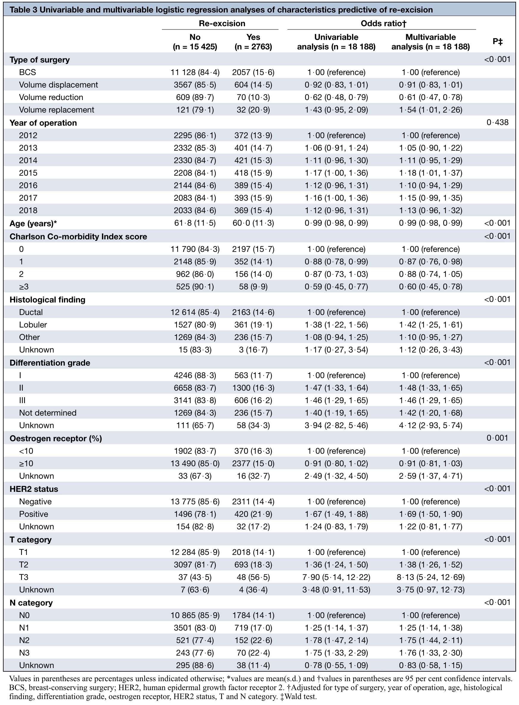
Final replica
Some personal comments:
- Univariable test results are as they are. MV analysis results are different than original because it is not easy to fabricate totally similar relationships among variables (at least for me).
- Wald test may not be needed in this analysis. They seem useless. Odds ratios with confidence intervals are good enough.
- Wald test results are different than the values presented in the original table. I do not know the reason, possibly my mistake (or authors), not sure.
Citation
Ali Guner (May 6, 2022) Week-9. Retrieved from https://datavizmed.com/blog/2022-05-06-week-9/
@misc{ 2022-week-9,
author = { Ali Guner },
title = { Week-9 },
url = { https://datavizmed.com/blog/2022-05-06-week-9/ },
year = { 2022 }
updated = { May 6, 2022 }
}